Immerse Yourself in Reinforcement Learning and Robotics with MujoCo
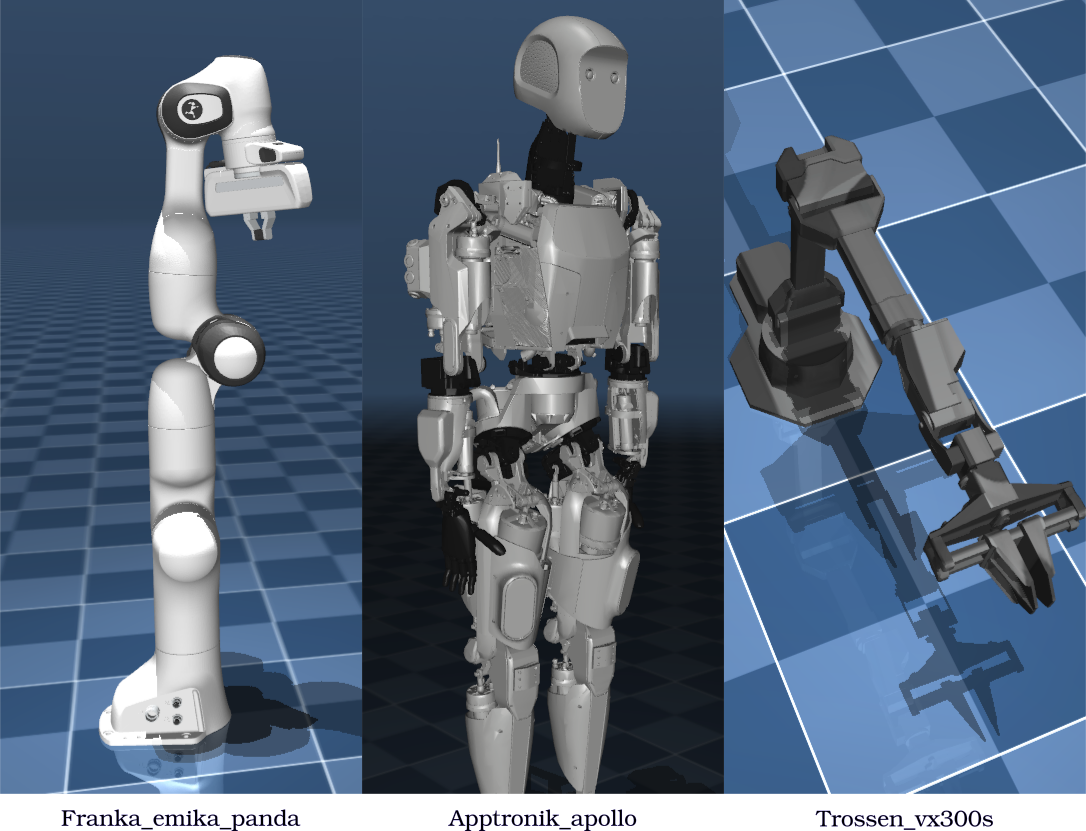
MujoCo is a physics simulator for robotics research developed by Google DeepMind and written in C++ with a Python API. The advantage of using MujoCo is due to its various implemented models along with full dynamic and physics properties, such as friction, inertia, elasticity, etc. This realism allows researchers to rigorously test reinforcement learning algorithms in simulations before deployment, mitigating risks associated with real-world applications. Simulating exact replicas of robot manipulators becomes particularly valuable, enabling training in a safe virtual environment and seamless transition to production. Notable examples include open-source models for popular brands like ALOHA, FRANKA, and KUKA readily available within MujoCo.
Table of Content:
- Overview
- MJCF Format
- The Task
- Continuous Proximal Policy Optimization
- Training Results
- Conclusion
Overview
Beyond the core MujoCo library (installable via pip install mujoco
), two invaluable packages enhance its capabilities: dm_control
(https://github.com/google-deepmind/dm_control) and mujoco_menagerie
(https://github.com/google-deepmind/mujoco_menagerie).
mujoco_menagerie
offers a wealth of open-source robot models in .xml
format, simplifying the simulation of complex systems. These models encompass diverse designs, as illustrated
below:

Images rendered from xml source in menagerie under BSD-3-Clause for Trossen, and Apache license for Franka and Apptronik
dm_control
(installable via pip install dm_control
) provides a robust framework for building Reinforcement Learning pipelines directly from MujoCo models. Its suite
subpackage offers pre-defined environments with standardized .step()
and .reward()
methods, serving as benchmarks for evaluating and comparing various RL algorithms.
These benchmarks can be shown by running the following:
# Control Suite from dm_control import suite for domain, task in suite.BENCHMARKING: print(f'{domain:<{max_len}} {task}')
which will give the following domains and tasks among others:
Domain | acrobot | ball_in_cup | cartpole | cheetah | finger | fish | hopper | humanoid |
---|---|---|---|---|---|---|---|---|
Tasks | swingup | catch | balance | run | spin | upright | stand | stand |
Additionally dm_control
allow the manipulation of the MJCF models of the entities from within the running script, utilizing its PyMJCF
subpackage. This eliminates the need to manually edit XML files for tasks such as adding new joints or replicating specific structures.
MJCF, short for MuJoCo XML Configuration File, serves as the foundation for representing physical entities in MujoCo. It defines bodies, joints, and their properties, dictating how objects interact within the simulation. Familiarity with this format is essential for effectively utilizing MujoCo. For a deeper understanding of MJCF syntax and functionalities, consult the comprehensive documentation and tutorial notebook provided by MuJoCo itself.
MuJoCo XML Configuration File Format (MJCF)
To illustrate the structure of an MJCF file, let's examine the car.xml
source code found within the MuJoCo GitHub repository. This example showcases a simple three-wheeled toy vehicle equipped with two front lights, featuring two primary degrees of freedom (DoFs): on the forward-backward movement and left-right turning.
Examining the initial portion of the code reveals that all elements reside within <mujoco>
and </mujoco>
tags, establishing the root element for the entire configuration. Notice the <compiler>
tag defining the simulation's integration method (Euler by default) and allowing for customization through its options.
<mujoco> <compiler autolimits="true"/>
When objects in your model require unique textures and geometries beyond standard shapes like spheres and boxes, leverage the <texture>
, <material>
, and <mesh>
tags. The <mesh>
tag, specifically, utilizes the vertex
option to define the precise coordinates of each point on the surface. Each row represents a single point.
<asset> <texture name="grid" type="2d" builtin="checker" width="512" height="512" rgb1=".1 .2 .3" rgb2=".2 .3 .4"/> <material name="grid" texture="grid" texrepeat="1 1" texuniform="true" reflectance=".2"/> <mesh name="chasis" scale=".01 .006 .0015" vertex=" 9 2 0 -10 10 10 9 -2 0 10 3 -10 10 -3 -10 -8 10 -10 -10 -10 10 -8 -10 -10 -5 0 20"/> </asset>
The <default>
tag streamlines your model by establishing default values for specific classes. For instance, the provided example defines a wheel
class with consistent shape (cylinder
), size (size
), and color (rgba
). This promotes efficient and organized code.
<default> <joint damping=".03" actuatorfrcrange="-0.5 0.5"/> <default class="wheel"> <geom type="cylinder" size=".03 .01" rgba=".5 .5 1 1"/> </default> <default class="decor"> <site type="box" rgba=".5 1 .5 1"/> </default> </default>
In Mujoco models, the <worldbody>
tag serves as the root object, designated with ID 0
, encompassing all other bodies within the model. As your example features a single car, its sole child body is named "car".
Within each body, you can further define its constituents using <body>
, <geom>
, <joint>
, and <light>
tags to represent additional bodies, geometries, joints, and lighting elements respectively.
This is illustrated in the following code snippet where we observe options like name
, class
, and pos
among others, which uniquely identify the element by name, assign it to a predefined class, often inherited from <default>
, and specify its initial position, respectively.
<worldbody> <geom type="plane" size="3 3 .01" material="grid"/> <body name="car" pos="0 0 .03"> <freejoint/> <light name="top light" pos="0 0 2" mode="trackcom" diffuse=".4 .4 .4"/> <geom name="chasis" type="mesh" mesh="chasis" rgba="0 .8 0 1"/> <geom name="front wheel" pos=".08 0 -.015" type="sphere" size=".015" condim="1" priority="1"/> <light name="front light" pos=".1 0 .02" dir="2 0 -1" diffuse="1 1 1"/> <body name="left wheel" pos="-.07 .06 0" zaxis="0 1 0"> <joint name="left"/> <geom class="wheel"/> <site class="decor" size=".006 .025 .012"/> <site class="decor" size=".025 .006 .012"/> </body> <body name="right wheel" pos="-.07 -.06 0" zaxis="0 1 0"> <joint name="right"/> <geom class="wheel"/> <site class="decor" size=".006 .025 .012"/> <site class="decor" size=".025 .006 .012"/> </body> </body> </worldbody>
As the car can move in any direction, including jumping and flipping, with respect to the ground floor, it gets <freejoint/>
tag with 6 DoFs.
While each of its wheels: right and left wheels, get one DoF, along its previously defined axis with the zaxis="0 1 0"
option, the y-axis.
MujoCo utilizes the <tendon>
tag to define control handles, grouping joints together. A <fixed>
tag then anchors these joint groups, followed by the <actuator>
tag which
specifies the exact name and control range of each motor associated with the tendon. A closer look at the code below demonstrates this structure.
<tendon> <fixed name="forward"> <joint joint="left" coef=".5"/> <joint joint="right" coef=".5"/> </fixed> <fixed name="turn"> <joint joint="left" coef="-.5"/> <joint joint="right" coef=".5"/> </fixed> </tendon> <actuator> <motor name="forward" tendon="forward" ctrlrange="-1 1"/> <motor name="turn" tendon="turn" ctrlrange="-1 1"/> </actuator>
This tendon-based system provides a flexible approach to controlling the car. For example, the "forward"
tendon governs linear movement, causing both wheels to displace forward by 0.5
simultaneously. The "turn"
tendon facilitates turning by applying opposite displacements to each wheel, resulting in a rotational motion.
The degree of displacement for each action is precisely controlled through the motors associated with each tendon by multiplying their values with the coef
values defined within the tendons.
Lastly, the <sensor>
tag defines the joints that should be sensed, returning their generalized displacements value on its DoF.
<sensor> <jointactuatorfrc name="right" joint="right"/> <jointactuatorfrc name="left" joint="left"/> </sensor> </mujoco>
The Task
To train and guide our reinforcement learning agent, we need to establish a clear objective – a specific behavior we want the car to exhibit. This could involve tasks like driving in a circular path or navigating towards a predetermined destination, even if its location is initially unknown.
For this example, let's define a rewarding scenario where the car travels from its starting position, A (0, 0, 0), to target position B (-1, 4, 0). As illustrated in the diagram below, point B lies to the left of the car's initial location, requiring it to both turn and drive in a straight line.

To effectively train our agent, we need a reward function that quantifies how well the car is performing its task. In this case, we'll base the reward on the Euclidean distance between the car's current position and target B.
We use the formula np.exp(-np.linalg.norm(A, B))
to represent this reward. By taking the exponent of the negative distance, we ensure that the reward values always fall within the range [0, 1]
. As the car gets closer to point B, the reward value increases, motivating the agent to continue its progress towards the target.
Continuous Proximal Policy Optimization (PPO)
Our chosen XML file specifies a continuous action space, with actuator values ranging from -1 to 1. This necessitates a training algorithm capable of handling continuous actions. While algorithms like DQN are suited for discrete action spaces, actor-critic methods such as PPO prove effective in this scenario.
The implementation utilizes the CleanRL
library single-file implementation for continuous PPO, modified to integrate our custom environment built around the existing MujoCo model. The training process involves 2 million steps, with each episode consisting of 2500 steps, equivalent to a duration of 5 seconds given MujoCo's default 2ms update rate.
A key distinction between discrete and continuous PPO lies in the policy model's output distribution. While discrete PPO employs a categorical distribution (Categorical
), continuous PPO utilizes a Gaussian (Normal
) or any other suitable continuous distribution.
The following section details the environment utilized for stepping and simulating the MujoCo model, which will be used for the training program of PPO.
Training Environment
As we will be using the main MujoCo package (not dm_control
), we will do the following imports:
import mujoco import mujoco.viewer import numpy as np import time import torch
The environment class's init
method establishes our simulation setup.
Firstly, we load the MuJoCo model from an XML file using mujoco.MjModel.from_xml_path()
. This provides us with the model structure, including geometries and essential constants like time steps and gravity, stored within model.opt
.
Next, we create a data
structure representing the current state of the simulation using data=mujoco.MjData(model)
. This structure holds crucial information such as generalized velocity (data.qvel
), generalized position (data.qpos
), and actuator values (data.ctrl
), allowing us to read and modify them throughout the simulation.
To ensure a realistic duration, we define the simulation time as 5 seconds. However, due to MuJoCo's fast simulation speed, this might be achieved in a shorter real-world time (e.g., 0.5 seconds). We can control the simulation pace by introducing delays accordingly.
Finally, if the render
variable is set to True
, we initialize a passive viewer GUI using mujoco.viewer.launch_passive(model,data)
. The "passive" feature prevents the GUI from blocking code execution while still updating with the latest values in data
when viewer.sync()
is called. Remember to close the viewer gracefully with viewer.close()
at the end.
class Cars(): def __init__(self, max_steps = 3*500, seed=0,render=False): self.model = mujoco.MjModel.from_xml_path('./car.xml') self.data = mujoco.MjData(self.model) self.duration = int(max_steps//500) self.single_action_space = (2,) self.single_observation_space = (13,) self.viewer = None self.reset() if render: self.viewer = mujoco.viewer.launch_passive(self.model, self.data)
Within reset()
, we strategically define the state variables our model will use for learning. Given that our task involves 2D movement, we select key parameters:
-
Position: The car's Cartesian coordinates (
data.body('car').xpos
) provide its location in the environment. -
Orientation: The car's quaternion representation (
data.body('car').xquat
) captures its rotational state, crucial for understanding its direction. -
Velocity: The car's linear velocity (
data.body('car').cvel
) informs us about its speed and direction of movement. This can be valuable for deciding whether to accelerate or decelerate.
Note that data.body()
or data.geom()
allow named access to these objects as defined in the XML file, or even by their index number , where 0
always indicate the worldbody
.
def reset(self): mujoco.mj_resetData(self.model, self.data) self.episodic_return = 0 state = np.hstack((self.data.body('car').xpos[:3], self.data.body('car').cvel, self.data.body('car').xquat)) if self.viewer is not None: self.viewer.close() self.viewer = mujoco.viewer.launch_passive(self.model, self.data) return state
To achieve our goal of reaching the target position [-1,4]
, we can define a reward function based on the distance between the current and desired positions. However, employing exp(-distance)
as the reward function proves more beneficial. This transformation restricts reward values to the range [0,1]
, promoting learning stability. Synchronizing changes to the viewer window is straightforward: simply invoke the command self.viewer.sync()
.
def reward(self, state, action): car_dist = (np.linalg.norm(np.array([-1,4]-state[:2]))) return np.exp(-((car_dist))) def render(self): if self.viewer.is_running(): self.viewer.sync() def close(self): self.viewer.close()
The step()
routine handles model updates. First, it sets the current action values for forward and turning movements within the data.ctrl
variable. However, these actions are subsequently transformed using np.tanh()
, ensuring an output range of [-1,1]
. This allows our policy neural network to be trained across the full range [-Inf, Inf]
, simplifying representation and mitigating potential rounding issues of small values during training. Additionally, we track episodic returns and manage terminal states by resetting the environment.
def step(self, action): self.data.ctrl = np.tanh(action) mujoco.mj_step(self.model, self.data) state = np.hstack((self.data.body('car').xpos[:3], self.data.body('car').cvel, self.data.body('car').xquat)) reward = self.reward(state, np.tanh(action)) self.episodic_return += reward done = False info = {} if self.data.time>=self.duration: done = True info.update({'episode':{'r':self.episodic_return,'l':self.data.time}}) info.update({"terminal_observation":state.copy()}) state = self.reset() return state, reward, done, info
This concludes the construction of our basic car model environment. While relatively straightforward, the dm_control
framework offers a wealth of pre-built environments and pipelines tailored for RL agent training. Exploring these advanced functionalities is left for future posts.
Training Results
After training our PPO agent within the previous MujoCo environment using a suitable network architecture, we observed the following episodic return curve:

The training curve clearly demonstrates the model's learning progress, albeit gradually. This marks the successful creation of our first simulated and controlled reinforcement learning agent within MujoCo!
To verify the agent's performance, we execute a separate testing program with the render
variable set to True
. This allows us to visually observe the agent's actions.
def main(): duration = 5 env = Cars(max_steps=duration*500,render=True) #2000000 is the training iterations policy = torch.load(f'ppo_agent_cars_{2000000}_mlp.pth') state = env.reset() start = time.time() while time.time() - start < duration: with torch.no_grad(): action = policy.actor(torch.Tensor(state).to('cuda')).cpu().numpy()[:2] state, reward, done, info = env.step(action) if done: break time.sleep(0.003) env.render() env.close()
The testing program initializes the environment, loads our trained PyTorch model, and retrieves the initial state by resetting the environment. Within a while
loop, we alternate between: 1) inferring the action from the trained actor model, and 2) advancing the environment based on the chosen action. Finally, each frame is rendered using env.render()
.
Running this program without any delay results in an extremely fast simulation, potentially making observation difficult. Additionally, depending on our while
loop condition, the program may execute repeatedly before completion. To address this, we introduce a time delay (time.sleep()
) to slow down the simulation and ensure observability. While multiple iterations might still occur before the specified duration
, they will be visible.
In my case, the code successfully depicts the car maneuvering precisely as illustrated in the The Task section. However, due to the limited speed and a 5-second episode length, the simulation concludes before reaching the target point [-1,4]
, as this will be physically impossible in that case, no matter how long the model is trained.
Conclusion
While this tutorial merely scratches the surface of MuJoCo's vast API capabilities, it equips you with the foundational knowledge to embark on your robotic simulation journey. MuJoCo's C++ foundation enables lightning-fast performance, making it ideal for training intricate robots of diverse configurations.
This versatility positions MuJoCo as a valuable tool in both research and industry:
- Research: Researchers can rigorously test and compare novel reinforcement learning algorithms within challenging, realistic scenarios without the logistical complexities and costs of physical prototyping.
- Industry: Manufacturers can thoroughly evaluate robot designs and models in environments mirroring real-world conditions, ensuring optimal performance before deployment.
This Reinforcement and Imitation Learning series will delve deeper into specific, popular algorithms, exploring their intricacies and applications. Subscribe or follow along to stay informed and explore the full potential of these powerful techniques!